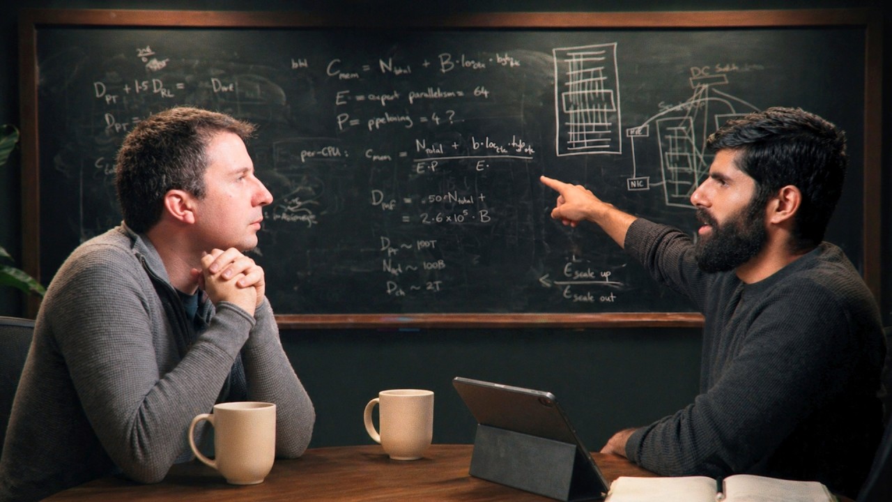
This episode is a blackboard lecture by Reiner Pope (CEO of MatX, former Google TPU architect) on how modern AI models are trained and served at scale. Using first-principles analysis, he explains how hardware constraints—memory bandwidth, compute throughput, memory capacity, and network topology—shape everything from model architecture and API pricing to the pace of AI progress. The core insight is that batch size is the single most important lever in inference economics, and that understanding roofline analysis (the tradeoff between memory-bound and compute-bound operation) explains why models are priced, sized, and parallelized the way they are.
Batch size is the key variable in inference cost and latency
When you serve a model, you don’t process one user at a time—you batch many users’ requests together. This is the single most important optimization in inference.
At batch size = 1, cost per token is astronomically high because you must fetch all model weights from memory for just one token. The weight-fetch time dominates.
As batch size increases, the fixed cost of fetching weights is amortized across many tokens, and cost per token drops sharply—eventually flattening out when compute time (not memory) becomes the bottleneck.
This creates a U-shaped cost curve: very expensive at low batch sizes, approaching a floor at high batch sizes. The floor is set by compute time alone (you must still do the matrix multiplies for each token).
Latency has a floor too: you cannot go faster than the time it takes to read all weights from memory into the chips. On current hardware (HBM), this is roughly 15–20 milliseconds—the time to “evacuate” all of HBM once.
This is why there’s a lower bound on latency regardless of batch size. You can’t beat the memory bandwidth wall.
Practical implication for “Fast Mode” vs “Slow Mode” APIs: Fast Mode (higher price, lower latency) corresponds to running with a smaller batch—you get your tokens sooner but pay more per token because weights aren’t amortized. Slow Mode (lower price, higher latency) corresponds to waiting for a larger batch to fill up, amortizing costs. But there’s a floor—you can’t get arbitrarily cheap by waiting longer, because eventually compute (not memory) dominates cost.
The optimal batch size is determined by hardware and model sparsity
The crossover point where memory time equals compute time gives the optimal batch size. Setting weight-fetch time equal to weight-multiply time yields:
Batch size ≈ 300 × sparsity ratio, where sparsity = active parameters / total parameters.
For DeepSeek V3 (37B active out of 700B total, sparsity ≈ 1/19, but with 8 out of 256 experts activated, sparsity = 8), this gives roughly 2,000–3,000 tokens per batch.
This number is remarkably stable across hardware generations because the FLOPs-to-bandwidth ratio of GPUs has stayed around 300 from A100 through B100.
Including KV cache in the calculation pushes the optimal batch size higher, because KV fetches consume memory bandwidth that could otherwise be used for weight loads.
Practical batch sizes are 2–3× the theoretical minimum because real-world efficiency is lower than roofline predictions.
At batch size ~2,000 and a 20ms cycle time, a single rack produces roughly 128,000 tokens/second. Global systems serve hundreds of millions of tokens/second, meaning even a “small” competitive deployment needs ~1/1000th of global capacity—still a significant scale.
Sparsity (Mixture of Experts) lets you trade compute for memory
Sparse MoE models activate only a fraction of their parameters per token. DeepSeek V3 has 700B total parameters but only 37B active per token.
This is a pure win from the analysis above: fewer active parameters means less compute per token, which means you can run at the compute-floor cost point with a smaller batch.
The cost is that total parameters still must be stored in memory (you might need any expert on any token), so memory capacity requirements grow.
Empirical quality trade-offs: Older papers (Switch Transformer, GShard) showed that a sparse model with more total parameters but the same active parameter count can match or exceed dense model quality. A 64-expert model with 370M activated parameters matched a 1.3B dense model—a 4× increase in total params for no loss in quality.
The trade-off is favorable because the extra memory cost is amortized across the batch, and the compute savings are real. You should keep increasing sparsity until you run out of users to batch (or hit memory capacity limits).
Modern techniques (DeepSeek’s finer-grained experts) have improved this further, but the fundamental trade-off remains empirical.
How MoE models are mapped onto GPU racks
Expert parallelism is the standard approach: different experts live on different GPUs. With 256 experts and 64 GPUs, each GPU holds 4 experts.
This creates an all-to-all communication pattern: any GPU may need to send tokens to any other GPU (depending on routing decisions). This is exactly what Nvidia’s NVLink topology within a rack is designed for—every GPU connects to a central switch, enabling all-to-all in two hops.
The rack boundary is a hard bottleneck: Communication between racks (scale-out) is roughly 8× slower than within a rack (scale-up). If experts are split across racks, half the traffic must traverse the slow inter-rack link, creating a bottleneck.
This means one rack bounds the size of an expert layer. You want all experts for a single MoE layer within one rack.
Why not build one giant switch? Cabling density, power delivery, weight, and cooling constrain rack size. Running twice as many cables into a rack requires physically doubling wire density, which runs into bend radius limits, connector density, and backplane constraints. Modern racks are already at extreme physical limits.
Nvidia went from 8 GPUs (Hopper) to 72 (Blackwell) by switching from trays to racks as the form factor. Going to ~500 (Rubin) requires genuinely new physical rack designs with more complex cabling.
Pipeline parallelism spreads layers across racks
Pipeline parallelism assigns different layers to different racks. Layer 1–25 on rack 1, layers 26–50 on rack 2, etc.
This is necessary when the model is too large to fit in one rack’s memory, or when you want to scale beyond a single scale-up domain.
Communication analysis: The key question is whether inter-rack communication becomes a bottleneck. The ratio of scale-up time to scale-out time depends on: (bandwidth ratio) × (number of activated experts) × (number of layers per stage) × (factor of 2 for all-to-all). With 8× bandwidth ratio, 8+ activated experts, and multiple layers per stage, it’s easy to keep scale-up time dominant—meaning pipeline parallelism works well.
The physical cutting of the model matches the logical architecture: experts are cut across GPUs, layers are cut across racks. This is not a coincidence—it’s the natural way to parallelize along the model’s existing dimensions.
Pipeline bubbles: In inference, pipeline bubbles are easily hidden by running multiple sequences through the pipeline simultaneously (like an assembly line). In training, you need micro-batching to avoid bubbles, which means the global batch size = micro-batch size × number of pipeline stages.
Ilya’s claim that “pipelining is not wise” reflects real costs: pipeline parallelism creates architectural constraints (residual connections spanning pipeline stages become hard to implement, as in Kimi’s architecture). But it does save memory capacity, which can be valuable.
Pipelining saves memory capacity but not KV cache memory
Pipelining divides both terms by the number of pipeline stages. But for the KV cache, the batch size per pipeline stage must increase to keep all stages busy (you need as many micro-batches as pipeline stages). The P’s cancel out for KV cache—you get no memory savings on KV cache from pipelining.
This is a fundamental result: KV cache cannot be amortized across batch (each sequence has unique KV) and cannot be sharded across pipeline stages (you need all stages busy simultaneously). KV cache is the memory bottleneck.
Implication: For most current models, a single Blackwell rack has enough memory (~10–20 TB) to hold even a multi-trillion-parameter model plus KV cache. Pipelining is useful for very large models or extremely long contexts, but it’s not a silver bullet.
Scale-up size matters most for memory bandwidth, not capacity
Why did model sizes stay flat for years? GPT-4 (rumored >1T parameters) was released in 2023, and significantly larger models only appeared ~6 months before this episode. The constraint wasn’t memory capacity (pipelining solves that) but memory bandwidth.
Weight-fetch time = total parameters / (scale-up size × per-GPU bandwidth). Increasing the scale-up domain from 8 GPUs (Hopper) to 72 (Blackwell) gives a 9× improvement in effective memory bandwidth, directly reducing latency.
This is why Gemini (Google, with large TPU scale-up domains for years) appeared to have an advantage—not just from sparsity, but from being able to serve larger models at acceptable latency.
Latency per rack hop is on the order of milliseconds. With 4 pipeline stages, that’s ~10ms additional latency per token—significant but manageable. The bigger benefit of larger scale-up is avoiding these hops entirely.
Models are ~100× over-trained beyond Chinchilla-optimal
Chinchilla scaling laws say the optimal training data for a model is ~20× the number of parameters. But inference-era models are trained on far more data than this.
Heuristic: Total cost = training cost + RL cost + inference cost. The minimum tends to occur when these three costs are roughly equalized.
Pre-training cost ≈ 6 × active_params × pre_training_data (the 6ND formula: 2 for forward, 4 for backward).
Inference cost ≈ 2 × active_params × inference_data (forward-only for user tokens).
Equalizing these: pre-training data ≈ RL data ≈ inference data (within factors of ~2–3).
Back-of-envelope: If a model serves ~50M tokens/second for 2 months, that’s ~200 trillion inference tokens. This implies ~200 trillion pre-training tokens—roughly 100× the Chinchilla-optimal amount for a frontier model.
This over-training makes sense because inference is cheap relative to training for a high-quality model. You’d rather train a smaller model longer (more tokens, fewer parameters) than train a larger model for fewer tokens, because the smaller model is cheaper to serve to millions of users.
You can deduce pre-training data from API prices and traffic: If you know how many tokens a lab serves and assume cost equalization, you can estimate how much data went into training.
API pricing reveals internal cost structures
Long-context pricing (e.g., Gemini 3.1 charging 50% more above 200K tokens): This 50% bump reveals the crossover point where KV cache memory time starts to dominate compute time. At 200K context, the memory time for fetching KV cache equals the compute time for matrix multiplies.
From this, you can solve for bytes per token in the KV cache: ~1,667 bytes (~2 KB). This is consistent with dense attention using shared KV across layers (Character AI-style alternating layers) with 8 KV heads and d_head=128.
Input vs. output pricing (input tokens 3–5× cheaper than output tokens): This reveals that decode is memory-bandwidth bound while prefill is compute-bound.
In decode (generating one token), you must fetch the entire KV cache for that one token—memory bandwidth dominates.
In prefill (processing a long prompt), you process many tokens in parallel, amortizing the KV cache fetch across many tokens. The cost per token drops, and compute dominates.
The 5× ratio tells you how far below the compute roof the decode path is operating—it’s heavily memory-bandwidth bottlenecked.
Cache hit pricing (10× cheaper than recomputation): This reveals the memory tier hierarchy.
Recomputing KV cache from scratch costs a full forward pass (compute-expensive). Storing it in HBM and reusing it is cheap.
The pricing for 5-minute vs. 1-hour cache retention (~1.25× price difference) maps to the drain time of different memory tiers: the time to read the entire capacity of that tier. HBM drains in ~20ms, DDR in seconds, flash in ~minutes, spinning disk in ~hours.
The 5-minute and 1-hour tiers likely correspond to flash and spinning disk respectively—hyperscalers are using spinning disk for long-tail KV cache storage.
Sparse attention and the memory wall limit context length
Context lengths have plateaued at ~100–200K tokens for the past 1–2 years. This is the “reasonably balanced cost point” where memory bandwidth cost starts to dominate.
The compute cost of attention grows quadratically with context length, but in practice the linear term dominates until millions of tokens. The real bottleneck is memory bandwidth (fetching KV cache) and memory capacity (storing it).
Sparse attention (e.g., DeepSeek’s mechanism) improves scaling from linear to square root, but it’s not infinite—attending to too sparse a subset of tokens degrades quality.
The memory wall: HBM bandwidth isn’t improving dramatically generation over generation. Without a breakthrough in memory technology or model architecture, context lengths won’t increase by orders of magnitude. This challenges the “in-context learning is enough for AGI” thesis, since human-level working memory might require ~100M token contexts.
Convergent evolution between neural networks and cryptography
Neural networks and cryptographic ciphers both need to mix information across all inputs, but in opposite directions:
Ciphers take structured input and make it look random (maximize entropy, avalanche property).
Neural networks take seemingly random input (text, DNA) and extract structure (minimize entropy, find patterns).
Shared mechanisms: Both use repeated layers of mixing operations. A randomly initialized neural network is actually a decent cipher—the problem is making it useful for computation (via gradient descent) rather than just scrambling.
Differential cryptanalysis (analyzing how small input changes affect output) is analogous to computing gradients. Ciphers are designed to maximize output difference; neural networks are designed to make gradients meaningful and stable (via residual connections, LayerNorm).
Cross-pollination: The Feistel network (a cipher construction that builds invertible functions from non-invertible components) was imported into neural networks as RevNets (2017).
RevNets make every layer invertible by keeping a copy of the input and swapping halves. This means you can rematerialize activations during the backward pass instead of storing them, dramatically reducing training memory at the cost of extra compute.
This is the inverse tradeoff of the KV cache: KV cache spends memory to save compute; RevNets spend compute to save memory. Given current hardware (memory is the bottleneck), KV cache is generally more profitable.